인공 신경망 분야에서 미니 배치는 대규모 데이터 세트로 신경망을 훈련시키는 데 사용되는 기술입니다. 한 번에 전체 데이터 세트로 네트워크를 교육하는 대신 데이터를 미니 배치라고 하는 작은 청크로 나누고 각 미니 배치에 대해 네트워크를 개별적으로 교육합니다.
목차
미니배치의 특징
신경망을 훈련할 때 예측된 출력과 원하는 출력 사이의 오류를 기반으로 네트워크의 가중치와 편향이 업데이트됩니다. 이 오차는 평균 제곱 오차와 같은 손실 함수를 사용하여 계산됩니다. 네트워크의 가중치와 편향은 오류를 줄이는 방향으로 업데이트됩니다. 이 프로세스를 역전파라고 합니다.
대규모 데이터 세트로 작업할 때 오류를 계산하고 전체 데이터 세트에 대한 가중치와 편향을 한 번에 업데이트하는 데 계산 비용이 많이 들 수 있습니다. 여기에서 미니 배치가 필요합니다. 전체 데이터 세트 대신 데이터의 작은 청크(미니 배치)로 네트워크를 훈련하면 계산 시간과 메모리 요구 사항을 줄일 수 있습니다.
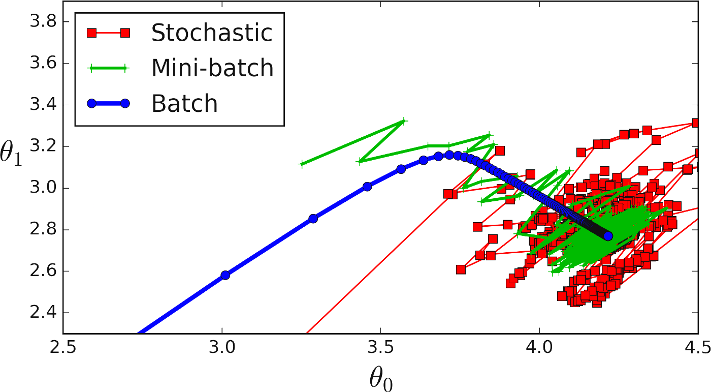
일반적인 미니 배치 크기는 32에서 256 사이입니다. 미니 배치 크기를 선택할 때 고려해야 할 몇 가지 장단점이 있습니다. 미니 배치 크기가 클수록 가중치 및 편향에 대한 업데이트가 적어지므로 네트워크가 더 빠르게 수렴됩니다. 그러나 더 많은 메모리와 계산 시간이 필요합니다. 미니 배치 크기가 작을수록 가중치와 편향이 더 많이 업데이트되므로 네트워크가 더 느리게 수렴됩니다. 그러나 메모리와 계산 시간도 적게 필요합니다.
요약하면 미니 배치는 대규모 데이터 세트로 신경망을 훈련하는 데 사용되는 기술입니다. 한 번에 전체 데이터 세트로 네트워크를 교육하는 대신 데이터를 미니 배치라고 하는 작은 청크로 나누고 각 미니 배치에 대해 네트워크를 개별적으로 교육합니다. 이것은 더 빠른 훈련과 더 적은 메모리 요구 사항을 허용합니다. 미니 배치 크기의 선택은 계산 시간과 메모리 요구 사항 및 업데이트 수 간의 균형입니다.
[컴퓨터과학/딥러닝] - 배치처리란 무엇인가? 인공신경망의 배치처리의 특징과 구현
미니배치 구현
import numpy as np

# Define the network's architecture
input_size = 2
hidden_size = 3
output_size = 1

# Initialize the weights and biases
weights = {
    'hidden': np.random.randn(input_size, hidden_size),
    'output': np.random.randn(hidden_size, output_size)
}
biases = {
    'hidden': np.random.randn(hidden_size),
    'output': np.random.randn(output_size)
}

# Define the activation function (sigmoid in this example)
def sigmoid(x):
    return 1 / (1 + np.exp(-x))

# Define the forward pass of the network
def forward(x, weights, biases):
    hidden_layer = np.dot(x, weights['hidden']) + biases['hidden']
    hidden_layer_output = sigmoid(hidden_layer)
    output_layer = np.dot(hidden_layer_output, weights['output']) + biases['output']
    output = sigmoid(output_layer)
    return output

# Define the backward pass (backpropagation)
def backward(x, y, weights, biases, output):
    # Calculate the error
    error = y - output

    # Calculate the gradient for the output layer
    output_layer_error = error * output * (1 - output)
    output_layer_gradient = np.dot(hidden_layer_output.T, output_layer_error)

    # Calculate the gradient for the hidden layer
    hidden_layer_error = np.dot(output_layer_error, weights['output'].T) * hidden_layer_output * (1 - hidden_layer_output)
    hidden_layer_gradient = np.dot(x.T, hidden_layer_error)

    # Return the gradients
    return {
        'hidden': hidden_layer_gradient,
        'output': output_layer_gradient
    }

# Define the training data
x = np.array([[1, 2], [2, 3], [3, 4], [4, 5], [5, 6], [6, 7], [7, 8], [8, 9], [9, 10], [10, 11]])
y = np.array([[0], [0], [1], [1], [1], [0], [0], [1], [1], [1]])

# Define the mini-batch size
batch_size = 2

# Initialize the number of iterations
num_iterations = 100

# Initialize the learning rate
learning_rate = 0.1

# Perform the forward and backward pass for each mini-batch
for iteration in range(num_iterations):
    for i in range(0, x.shape[0], batch_size):
        x_batch = x[i:i+batch_size]
        y_batch = y[i:i+batch_size]
        output = forward(x_batch, weights, biases)
        gradients = backward(x_batch, y_batch, weights, biases, output)

        # Update the weights
관련 글
'컴퓨터과학/딥러닝' 카테고리의 글 목록
모든 분야의 정보를 담고 있는 정보의 호텔입니다. 주로 컴전기입니다.
jkcb.tistory.com